![]()
There are many ways in Excel to
define data in a cell (typing being the most obvious), but sometimes we
want that value to be from a predefined list.
Excel does provide the ability to validate the number against values
appearing in a range of cells - the validate option.
This option requires the number to be manually entered first, issuing a
message if the value is incorrect -it's also rather cumbersome to set
up.
A better, and altogether more professional looking approach is to use drop down boxes.

The big advantage of this approach is that user simply clicks on the
down arrow to enable selection, then scroll down the list to select
their required value. They can't select an invalid value, because
they're limited to values in the range, the look and feel is the same
as Excel and it looks like a professional Excel adaptation, without any
programming code or macros.
To add a drop down box to a spreadsheet, first display the control toolbox (View, Toolbars, Control Toolbox).
Next click on the Combo box icon
 (this can also be located by hovering the cursor over icons until you see the "Combo box" note).
The cursor image will change (to cross-hairs),
and you may choose where to drop the control.
When you enabled the control toolbox, the macro toolbar probably appeared at the same time.
This should have the design icon
 button
depressed - if not click it. This enables changes to the properties of
the control by clicking on it (rather than just showing a blank
pull-down list).
button
depressed - if not click it. This enables changes to the properties of
the control by clicking on it (rather than just showing a blank
pull-down list).
Now right click against the tool, and select Properties. A form full of options will appear - scroll down to linked cell.
The linked cell is where Excel will place the selection made, and which can be used in your VLOOKUPs.
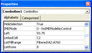
Next, select List Fill Range, and enter the location of the list of
values in your spreadsheet which a user may choose from.
The properties form does not allow you to click and drag to define the
range, like it does with function boxes, so sometimes ranges can be
simpler to define outside of the properties window by entering part of
a function (eg. '=SUM('), then clicking and dragging to define the
range and finally copying the range displayed too the clipboard - this
is especially true for ranges appearing on other sheets.
The definition of the control is now complete, and may be enabled by clicking on the design icon
again. You may have noticed that View
code was an option presented when you right clicked the control - this
would have allowed you to underpin the button with a Visual Basic
Macro, but we don't need any of that for the base functionality of the
control.
You may also notice that the
user selection now appears twice on your form, once on the button
itself, and oncee in the linked cell. Sometimes it's preferable to may
the linked cell invisible by changing it's colour, or actually moving
the control toolbox on top of it.
You can choose whether to print the image of the control or not, by right clicking, choosing Format Control, and ticking the Print image box.