![]()
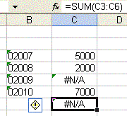
If the matrix of values comes from other calculations, such as VLOOKUPs, we sometimes find that one value is missing, and has #N/A in the cell. This error propagates to the SUM function, causing that to display #N/A too. This can be useful in that it may alert us that a value hasn't been found, and we can then fix the problem (possibly using the VLOOKUP assistant). It can also be a complete pain when we know that value is missing, and we just want the total of the rest.
The Fix #N/A macro will ignore any cells that Excel flags as an error, treating them as blanks. An example of such an error is shown below ;
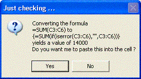
Clicking yes would change the new formula into the cell, fixing the problem. Note that the double quotes shown in the middle of the new formula means treat the erroneous cells as blanks. We could change this to zero, but bear in mind that this may have an implications if we were using a function like AVERAGE. The AVERAGE function would ignore blanks completely, making the average of the numbers shown in the example above (5000+2000+7000)/3, whereas using zero would calculate the average as (5000+2000+0+7000)/4. Dividing the result by 4 and not 3.
If you do alter the formula again, you'll need to press Control, Shift, and Enter rather than just error to preserve the new functionality. That is because the new formula is an array style formula (see below for details).
The formula has been modified and changed to an array style formula. In these kinds of formulae, each value in a range is evaluated in the condition separately, the result going into the surrounding formula. So in the example above, the IF function is evaluated against ISERROR(C3) first, returning C3 in this case, because C3 is not in an error state. The same test is applied against each cell in the range C3:C6, then the values return are substituted into the SUM function as SUM(5000,2000,"",7000).
There are many more examples of array functions on the web.